Image Based Lighting: Part 2 (Specular IBL)

As we have completed the diffuse irradiance component of IBL, we will move on to the specular part of the reflectance equation, as shown below.

\[\begin{align*} L_o(p, \omega_o) = \int_{\Omega} \left( k_s \frac{DFG}{4(\omega_o \cdot n)(\omega_i \cdot n)} \right) L_i(p, \omega_i) (n \cdot \omega_i) \, d\omega_i \end{align*}\]

Here if we observe, we will find that the Cook-Torrance component of the reflectance equation is not constant over the integral, unlike the diffuse component. It depends on both the incoming light direction and the view direction. Solving this integral for both variables is computationally expensive and even precomputing for both will not be practical in real-time setting. A standard approach is to split the specular integral into two parts, which can be convoluted separately.

If we rewrite the specular component of the reflectance equation as follows:

\[\begin{align*} L_o(p, \omega_o) = \int_{\Omega}f_r(p, \omega_i, \omega_o)\, L_i(p, \omega_i) (n \cdot \omega_i) \, d\omega_i \end{align*}\]

and then split it into two different separate Integrals like this:

\[\begin{align*} L_o(p, \omega_o) = \int_{\Omega}L_i(p, \omega_i)\, d\omega_i * \int_{\Omega}f_r(p, \omega_i, \omega_o)(n \cdot \omega_i) \, d\omega_i \end{align*}\]

After convolution, the first integral becomes the pre-filtered environment map, and the second becomes the BRDF integration map.

Pre filtered environment map

Prefiltering an environment map is similar to the convolution process for the irradiance map in diffuse IBL, except that we account for roughness here. With each increasing roughness levels, we will convolute it with more scattered vectors which will result in more blurrier reflections. Each roughness level result will be stored in the mipmap levels of prefiltered environment map.

In irradiance convolution, sample vectors were generated uniformly over the hemisphere using spherical coordinates. For specular reflection, when roughness is considered, outgoing vectors are more scattered and do not follow a specific direction or angle. The general shape of outgoing light reflections is known as the specular lobe. The size of the specular lobe depends on the roughness. We can assume that this lobe will define the reflection orientation around the halfway vector for a given incoming light direction. With this, it’s better to generate the sample vectors which are part of this specular lobe because other outgoing rays will not contribute much. This process is known as importance sampling. We could have implemented this approach for diffuse irradiance calculation as well, by selecting the sample vectors which contributes significantly to the scene’s radiance.

For specular IBL, importance sampling will be performed using the Monte Carlo Integration method, which will help in computing the integral value with a limited number of sample vectors. This approach approximates the result of integrating over all possible sample vectors, which would otherwise be computationally infeasible. We can think of importance sampling as prioritizing key contributors for an output, ensuring the end result is achieved efficiently without wasting effort on less impactful elements.

This concept can be understood through a Normal Distribution, which is commonly observed in various aspects of life. In other parts of life too, most of the things are normally distributed. A lot of things are average, the frequency of averages will always be higher, the extremes are rare. Thus, by focusing on averages rather than extremes, a practical and efficient solution can be achieved.

We will follow the same steps we did in irradiance map calculation. We will start a loop over sampleCount and follow the standard method of generating a pseudo-random 2D vector Xi which will be used in Importance sampling to sample directions for reflection vectors based on surface roughness. While this may not produce evenly distributed sample vectors, it can yield visually similar results. Next, the mip level is calculated based on the input roughness and the GGX Distribution. It will ensure that rough surfaces will sample lower resolution mipmap levels, simulating the blurring effect for rough reflections. The environment map is then prefiltered based on the calculated mip level and stored in the prefilteredColor result. Finally, the result is divided by totalWeight to ensure that smaller NdotL values contribute less to the final result, while larger values contribute more. If we don’t do it, it can result in overly bright or dark reflections.

#version 430 core

in vec3 localPos;
out vec4 FragColor;

uniform samplerCube environmentMap; // Input high-resolution cubemap
uniform float roughness; // Roughness for current mipmap level

const float PI = 3.14159265359; 

// GGX Importance Sampling for hemisphere
vec3 ImportanceSampleGGX(vec2 Xi, vec3 N, float roughness) {
    float a = roughness * roughness;
    float a2 = a * a;

    // Spherical coordinates for sampling hemisphere
    float phi = 2.0 * PI * Xi.x; // Azimuthal angle (Xi.x is in range [0, 1))
    float cosTheta = sqrt((1.0 - Xi.y) / (1.0 + (a2 - 1.0) * Xi.y)); // Polar angle based on GGX distribution
    float sinTheta = sqrt(1.0 - cosTheta * cosTheta);

    // Cartesian coordinates in tangent space
    vec3 H = vec3(
        sinTheta * cos(phi), // x
        sinTheta * sin(phi), // y
        cosTheta             // z
    );

    // Transform H to world space using TBN matrix
    vec3 tangent = abs(N.z) < 0.999 ? vec3(0.0, 0.0, 1.0) : vec3(1.0, 0.0, 0.0); // Arbitrary tangent vector
    vec3 bitangent = normalize(cross(N, tangent)); // Bitangent vector
    mat3 TBN = mat3(tangent, bitangent, N);        // Tangent-to-world matrix

    return normalize(TBN * H); // Return normalized sample direction in world space
}
void main() {
    vec3 N = normalize(localPos); // Surface normal
    vec3 R = N; // Reflection vector
    vec3 V = R; // View direction (aligned with reflection)

    const int sampleCount = 1024;   // Number of samples
    vec3 prefilteredColor = vec3(0.0); 
    float totalWeight = 0.0;

    for (int i = 0; i < sampleCount; ++i) {
        // Generate random sample direction using GGX importance sampling
        vec2 Xi = vec2(
            fract(sin(float(i) * 12.9898) * 43758.5453), // Random value 1
            fract(sin(float(i + 1) * 78.233) * 12345.6789) // Random value 2
        ); 

        vec3 H = ImportanceSampleGGX(Xi, N, roughness); // Halfway vector in world space
        vec3 L = normalize(reflect(-V, H)); // Reflect view direction over H

        // Weight based on the alignment of N and L
        float NdotL = max(dot(N, L), 0.0);
        if (NdotL > 0.0) {
            // sample from the environment's mip level based on roughness/pdf
            float D   = DistributionGGX(N, H, roughness); // standard PDF from PBR blog
            float NdotH = max(dot(N, H), 0.0);
            float HdotV = max(dot(H, V), 0.0);
            float pdf = D * NdotH / (4.0 * HdotV) + 0.0001; 

            float resolution = 512.0;
            float saTexel  = 4.0 * PI / (6.0 * resolution * resolution); // solid angle per texel, 4*PI because of cubemap and 6 faces
            float saSample = 1.0 / (float(sampleCount) * pdf + 0.0001); // solid angle per sample

            float mipLevel = roughness == 0.0 ? 0.0 : 0.5 * log2(saSample / saTexel);  
            
            prefilteredColor += textureLod(environmentMap, L, mipLevel).rgb * NdotL; // Accumulate reflected color
            totalWeight += NdotL; // Accumulate weight
        }
    }
    if (totalWeight > 0.0) {
        prefilteredColor = prefilteredColor / totalWeight; // Normalize color by total weight
    }
    FragColor = vec4(prefilteredColor, 1.0); // Output prefiltered color
}

Now, we can start writing the GeneratePrefilteredCubemap function, which is similar to GenerateIrradianceMap, but generates the map for multiple mipmap levels. I will paste the entire function below and highlight the differences in the code comments.

GLuint TextureUtilities::GeneratePrefilteredCubemap(GLuint& cubemapTexture, Shader& prefilterShader, GLuint maxMipLevels)
{
    GLuint prefilteredCubemap;
    glGenTextures(1, &prefilteredCubemap);
    glBindTexture(GL_TEXTURE_CUBE_MAP, prefilteredCubemap);

    for (GLuint i = 0; i < 6; ++i) {
        // for all mimmap levels
        for (GLuint mip = 0; mip < maxMipLevels; ++mip) {
            GLuint mipWidth = 128 >> mip;
            GLuint mipHeight = 128 >> mip;
            glTexImage2D(GL_TEXTURE_CUBE_MAP_POSITIVE_X + i, mip, GL_RGB16F, mipWidth, mipHeight, 0, GL_RGB, GL_FLOAT, nullptr);
        }
    }

    glTexParameteri(GL_TEXTURE_CUBE_MAP, GL_TEXTURE_WRAP_S, GL_CLAMP_TO_EDGE);
    ...
    glTexParameteri(GL_TEXTURE_CUBE_MAP, GL_TEXTURE_MIN_FILTER, GL_LINEAR_MIPMAP_LINEAR);
    ...

    glGenerateMipmap(GL_TEXTURE_CUBE_MAP); // to allocate the memory

    GLuint captureFBO, captureRBO;
    glGenFramebuffers(1, &captureFBO);
    glGenRenderbuffers(1, &captureRBO);

    prefilterShader.Activate();
    glActiveTexture(GL_TEXTURE0);
    glBindTexture(GL_TEXTURE_CUBE_MAP, cubemapTexture);
    glUniform1i(glGetUniformLocation(prefilterShader.ID, "environmentMap"), 0);

    for (GLuint mip = 0; mip < maxMipLevels; ++mip) {
        // reducing dimensions for each mipmap levels by scale of 2
        GLuint mipWidth = 128 >> mip;
        GLuint mipHeight = 128 >> mip;

        glViewport(0, 0, mipWidth, mipHeight);

        glBindRenderbuffer(GL_RENDERBUFFER, captureRBO);
        glRenderbufferStorage(GL_RENDERBUFFER, GL_DEPTH_COMPONENT24, mipWidth, mipHeight);
        glBindFramebuffer(GL_FRAMEBUFFER, captureFBO);

        float roughness = (float)mip / (float)(maxMipLevels - 1); // Roughness corresponds to mip level
        glUniform1f(glGetUniformLocation(prefilterShader.ID, "roughness"), roughness);

        for (GLuint i = 0; i < 6; ++i) {
            glFramebufferTexture2D(GL_FRAMEBUFFER, GL_COLOR_ATTACHMENT0, GL_TEXTURE_CUBE_MAP_POSITIVE_X + i, prefilteredCubemap, mip);
            glClear(GL_COLOR_BUFFER_BIT | GL_DEPTH_BUFFER_BIT);

            glUniformMatrix4fv(glGetUniformLocation(prefilterShader.ID, "camMatrix"), 1, GL_FALSE, glm::value_ptr(cameraMatrix[i]));
            // Render the cube using the Mesh class
            skymap->Draw(prefilterShader);
        }
    }

    glBindFramebuffer(GL_FRAMEBUFFER, 0);
    return prefilteredCubemap;
}

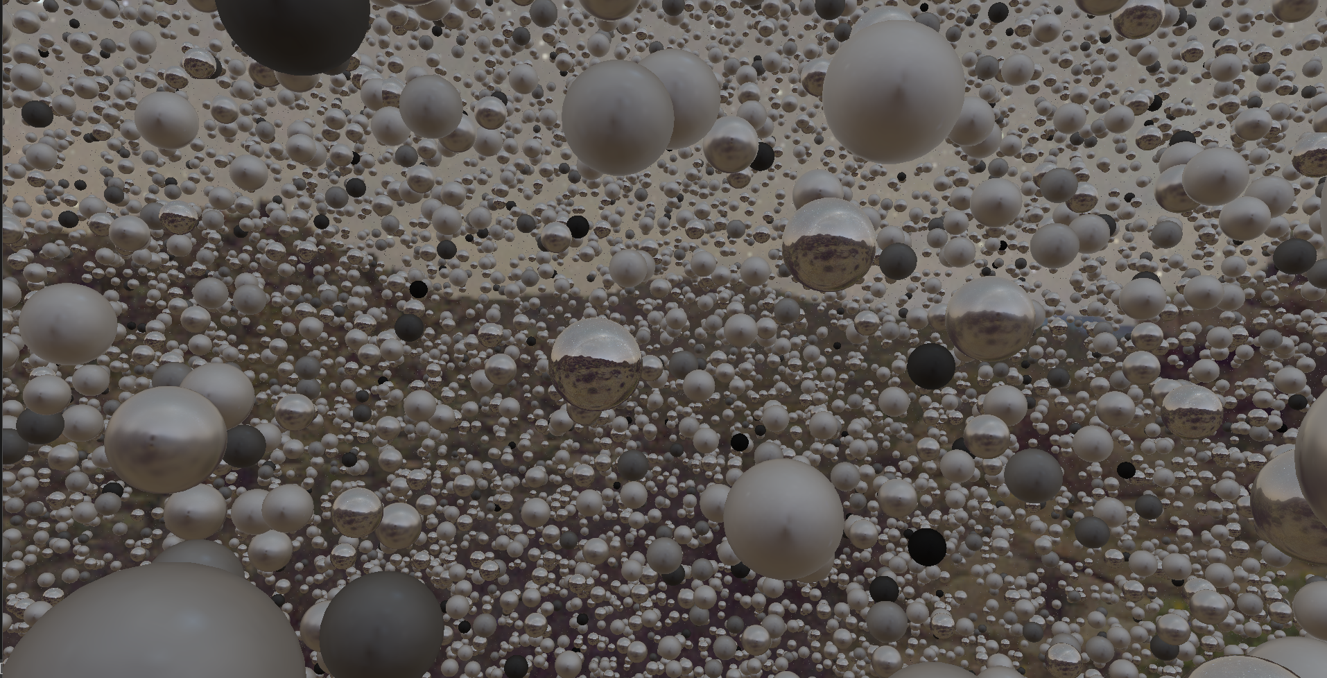
It Should produce output similar to the following. I have not yet explained how this will be integrated into the main fragment shader, but since I have already written that part, I’m showing this output.

BRDF Integration map

Next, we calculate the second integral $\int_{\Omega}f_r(p, \omega_i, \omega_o)(\mathbf{n} \cdot \omega_i) \, d\omega_i$. It requires convoluting the BRDF equation over the angle $\mathbf{n}.\omega_o$, the surface roughness and Fresnel’s $F_0$.

Convoluting over three variables is computationally intensive, so we will simplify the equation by extracting $F_0$ from it.

\[\begin{align*} \int_{\Omega}f_r(p, \omega_i, \omega_o)(n \cdot \omega_i) \, d\omega_i = \int_{\Omega} \frac{f_r(p, \omega_i, \omega_o)}{F(\omega_o, h)}F(\omega_o, h) (n \cdot \omega_i) \, d\omega_i \\ \end{align*}\]

Substituting the right most $F$ with Fresnel-Schlick approximation:

\[\begin{align*} \int_{\Omega}f_r(p, \omega_i, \omega_o)(n \cdot \omega_i) \, d\omega_i = \int_{\Omega} \frac{f_r(p, \omega_i, \omega_o)}{F(\omega_o, h)} (F_0 + (1-F_0)(1-w_o.h)^5) (n \cdot \omega_i) \, d\omega_i \\ =\int_{\Omega} \frac{f_r(p, \omega_i, \omega_o)}{F(\omega_o, h)} (F_0 * (1- (1-w_o.h)^5)+(1-w_o.h)^5) (n \cdot \omega_i) \, d\omega_i\\ \end{align*}\]

Next, split this integral into two parts:

\[\begin{align*} F_0\int_{\Omega} \frac{f_r(p, \omega_i, \omega_o)}{F(\omega_o, h)} (1- (1-w_o.h)^5)(n \cdot \omega_i) \, d\omega_i + \int_{\Omega} \frac{f_r(p, \omega_i, \omega_o)}{F(\omega_o, h)}(1-w_o.h)^5)(n \cdot \omega_i) \, d\omega_i \\ \end{align*}\]

This way, $F_0$ becomes constant over the integral, allowing us to remove it from the integration. If you remember the term $f_r(p, \omega_i, \omega_o)$ also contains $F$, so, it will get cancelled out in the equation.

Now, we will convolute it in same way we did for other convoluted environment maps. The key difference is that, instead of using a cubemap, we will use a 2D lookup texture called the BRDF integration map to store the convoluted result. This map will be used to calculate the final specular IBL result.

In the vertex shader, we pass the texture coordinates (texCoords) along with the local position. The fragment shader code is similar to prefilterShader, but processes the sample vectors based on the Geometry function and Fresnel-Schlick approximation.

...
float GeometrySchlickGGX(float NdotV, float roughness) {
    float r = roughness;
    float k = (r * r) / 2.0; // for IBL, k is different
    return NdotV / (NdotV * (1.0 - k) + k);
}
float GeometrySmith(vec3 N, vec3 V, vec3 L, float roughness)
{
    float NdotV = max(dot(N, V), 0.0);
    float NdotL = max(dot(N, L), 0.0);
    float ggx1 = GeometrySchlickGGX(NdotV, roughness);
    float ggx2 = GeometrySchlickGGX(NdotL, roughness);
    return ggx1 * ggx2;
}

vec2 IntegrateBRDF(float NdotV, float roughness) {
    const uint SAMPLE_COUNT = 2048u;
    vec3 V;
    V.x = sqrt(1.0 - NdotV * NdotV); // x can be calculated using pythagorean theorem
    V.y = 0.0; // vector lies on the xz-plane
    V.z = NdotV; // z-coordinate to cosine of angle between N and V

    float A = 0.0;
    float B = 0.0; 

    vec3 N = vec3(0.0, 0.0, 1.0); // Normal coming out of screen
        
    for(uint i = 0u; i < SAMPLE_COUNT; ++i) {
        vec2 Xi = vec2(float(i) / float(SAMPLE_COUNT), fract(sin(float(i) * 12.9898) * 43758.5453123)); // random values to generate random sample vector
        vec3 H = ImportanceSampleGGX(Xi, N, roughness); // halfway vector
        vec3 L = normalize(2.0 * dot(V, H) * H - V); // reflection of V about H

        float NdotL = max(L.z, 0.0); // cosine of angle between N and L, L.z used as N is aligned with z-axis
        float NdotH = max(H.z, 0.0); // similar to NDL
        float VdotH = max(dot(V, H), 0.0); // dot product of V and H

        if(NdotL > 0.0) {
            float G = GeometrySmith(N, V, L, roughness); // Geometry term
            float G_Vis = (G * VdotH) / (NdotH * NdotV + 0.001); // Visibility term combining geometry and Fresnel effects
            float Fc = pow(1.0 - VdotH, 5.0); // Fresnel Term

            A += (1.0 - Fc) * G_Vis;
            B += Fc * G_Vis;
        }
    }

    A /= float(SAMPLE_COUNT);
    B /= float(SAMPLE_COUNT);
    return vec2(A, B);
}

void main() 
{
    vec2 uv = TexCoords;
    float NdotV = uv.x; // x-axis will define the n.w_o
    float roughness = uv.y; // y-axis defining roughness
    vec2 integratedBRDF = IntegrateBRDF(NdotV, roughness);
    FragColor = integratedBRDF;
}

Now, we will generate a BRDF 2d Lookup texture with dimensions 512 x 512.

void RenderQuad() {
    static GLuint quadVAO=0, quadVBO;

    if (quadVAO == 0) {
        float quadVertices[] = {
            // Positions        // TexCoords
            -1.0f,  1.0f, 0.0f, 0.0f, 1.0f,
            -1.0f, -1.0f, 0.0f, 0.0f, 0.0f,
             1.0f,  1.0f, 0.0f, 1.0f, 1.0f,
             1.0f, -1.0f, 0.0f, 1.0f, 0.0f,
        };
        ...
        // VBO and VAO setup
        ...
        glEnableVertexAttribArray(0);
        glVertexAttribPointer(0, 3, GL_FLOAT, GL_FALSE, 5 * sizeof(float), (void*)0);
        ... // similarly for texCoords
        ...
    }

    glBindVertexArray(quadVAO);
    glDrawArrays(GL_TRIANGLE_STRIP, 0, 4); // Render fullscreen quad
    glBindVertexArray(0);
    //glDeleteVertexArrays(1, &quadVAO);
    //glDeleteBuffers(1, &quadVBO);
}
GLuint TextureUtilities::GenerateBRDFLUT(Shader& brdfShader)
{
    GLuint brdfLUTTexture;
    glGenTextures(1, &brdfLUTTexture);
    glBindTexture(GL_TEXTURE_2D, brdfLUTTexture);

    glTexImage2D(GL_TEXTURE_2D, 0, GL_RG16F, 512, 512, 0, GL_RG, GL_FLOAT, NULL); // allocating memory for BRDF LUT texture, see we are using GL_RG16F not including the B (or z) part, you can also use GL_RG32F

    // Set texture parameters
    glTexParameteri(GL_TEXTURE_2D, GL_TEXTURE_WRAP_S, GL_CLAMP_TO_EDGE);
    ...
    
    glViewport(0, 0, 512, 512);
    // Create framebuffer for BRDF LUT generation
    GLuint captureFBO, captureRBO;
    glGenFramebuffers(1, &captureFBO);
    glGenRenderbuffers(1, &captureRBO);

    glBindFramebuffer(GL_FRAMEBUFFER, captureFBO);
    glBindRenderbuffer(GL_RENDERBUFFER, captureRBO);
    glRenderbufferStorage(GL_RENDERBUFFER, GL_DEPTH_COMPONENT24, 512, 512);
    glFramebufferTexture2D(GL_FRAMEBUFFER, GL_COLOR_ATTACHMENT0, GL_TEXTURE_2D, brdfLUTTexture, 0);

    // Ensure framebuffer is complete
    if (glCheckFramebufferStatus(GL_FRAMEBUFFER) != GL_FRAMEBUFFER_COMPLETE) {
        std::cerr << "Framebuffer is not complete for BRDF LUT!" << std::endl;
        glBindFramebuffer(GL_FRAMEBUFFER, 0);
        return 0;
    }

    // Render quad using BRDF LUT shader
    brdfShader.Activate();
    glClear(GL_COLOR_BUFFER_BIT | GL_DEPTH_BUFFER_BIT);
    RenderQuad();
 
    glBindFramebuffer(GL_FRAMEBUFFER, 0);
    return brdfLUTTexture;
}

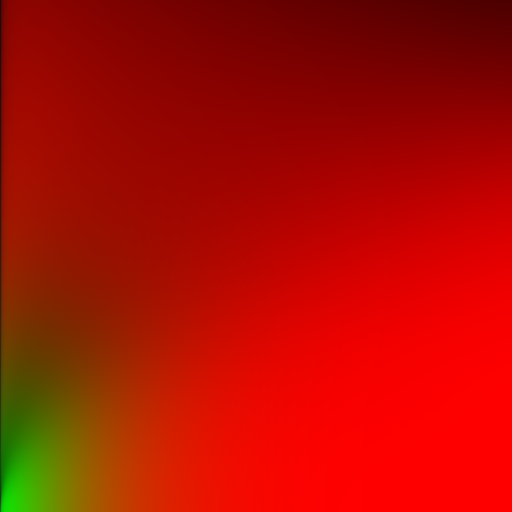
It should produce a new texture like following image.

Completing the specular IBL part of PBR shader

Both the prefilteredEnvMap and the brdfLUT map are passed to the shader as uniforms. To compute the specular reflections of the surface, we will sample the prefilteredEnvMap using the reflection vector based on the surface roughness and mip level, giving rough surface a blurrier reflection. Next, the BRDF LUT is sampled using the roughness and the angle between N (surface normal) and V (view direction).

...
// SPECULAR IBL
float roughnessLevel = ROUGHNESS * 4.0; 
vec3 prefilteredColor = textureLod(prefilteredEnvMap, R, roughnessLevel).rgb;
vec2 brdf = texture(brdfLUT, vec2(max(dot(N, V), 0.0), ROUGHNESS)).rg;
vec3 specularIBL = prefilteredColor * (F * brdf.x + brdf.y);

// combine diffuse and specular ibl
vec3 ambientIBL = (kD * diffuseIBL + specularIBL) * ao;
...
vec3 color = ambientIBL + directLighting;

// Gamma correction
color = color / (color + vec3(1.0));
color = pow(color, vec3(1.0/2.2));

FragColor = vec4(color, 1.0);

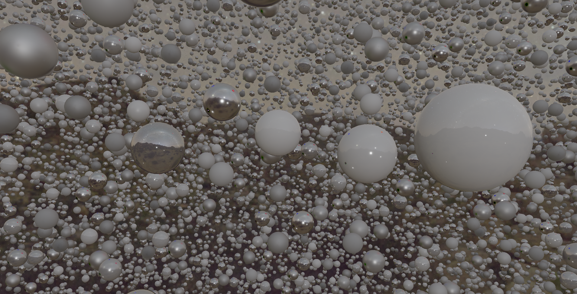
This produces the output shown below, fully implementing and visualizing Physically Based Rendering (PBR) with direct lighting and Image Based Lighting (IBL).

When the input Albedo color is also added, the output appears as shown below.

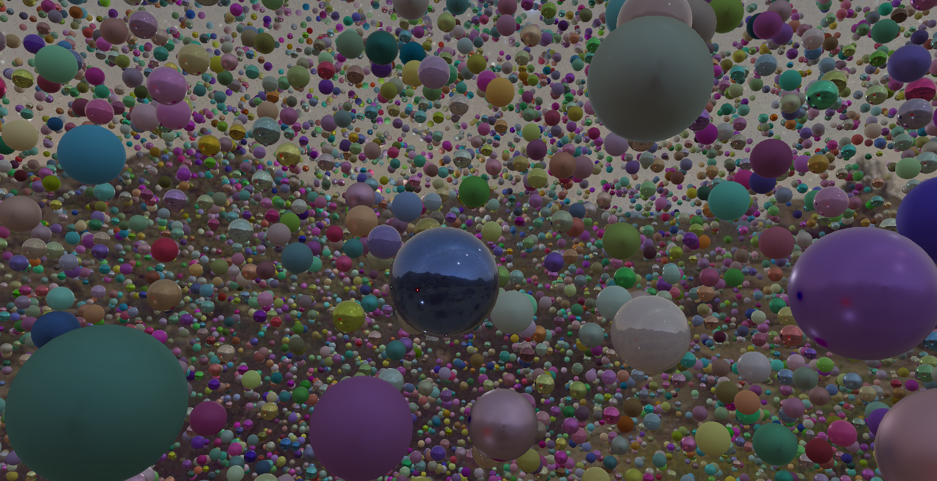
Final stats (per frame)

• Number of Draw calls: 4 (3 for sphere LODs, 1 for skybox)
• Total number of vertices: around 217 Million
• Compute shader time (in GPU): 0.25ms
• High detailed spheres draw time: 2.99ms
• Medium detailed spheres draw time: 8.04ms
• Low detailed spheres draw time: 2.12ms

With this, we have achieved our goal of rendering 1 Million spheres with dynamic lighting and Physically Based Rendering while maintaing 60fps on the screen.